Next: Histogram Bezier / Curves Up: Video Effects Previous: HistEQ Contents Index
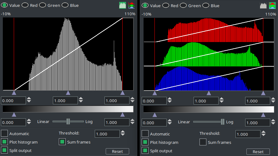
The histogram allows an immediate view of the contrast amplitude of an image with its distribution of luma and colors values. If the columns of values occupy the whole range 0 - 1.0 (also expressed as a percentage above the graph) then we have maximum contrast; if the range is smaller the contrast is smaller. In fact, contrast is mathematically given by the highest value of the abscissa minus the lowest value. If the values are similar and close together, the difference is smaller and the lower the contrast. If most of the values are on the right of the histogram you have an image with highlights at the limit with values clamped to 1.0. This is called overexposure. However, if most of the values are moved to the left, with the limit of the values clamped to 0, we have a lowlight image and we talk about underexposure. This plugin is a tool for Primary Color Correction, that is, affecting the entire frame. Histogram is keyframable (figure 10.50).
The Histogram is always performed in floating point RGB regardless of the project color space, but with clipping at 1.0. When using the X11 graphics driver and RGBA-FLOAT color model, Histogram allows you to display greater than (0 - 1.0f) values to accomodate HDR. This does not work when using X11-OpenGL because it is an 8-bit limited driver. The display will stop at +110%, but there is no clipping. By lowering the brightness all out-of-range values become visible, even those initially above 110%.
The histogram has two sets of transfer parameters: the input transfer and the output transfer. The input transfer has value on the horizontal axis of x; it is a normalized scale of values ranging from 0 - 1.0 (which for a depth color of 8 bits corresponds to the range 0 - 255, for 10 bits corresponds to 0 - 65536, etc). The output transfer (the yaxis) represents the height of the column where a given value x appears. A higher column (y greater) indicates that many pixels have the corresponding value x; a lower column indicates that fewer pixels have that value. On the left we have the minimum value 0, which is the black point. On the right we have the maximum value 1.0 which is the white point. The intermediate values pass smoothly from one extreme to the other. The three important points (including the midtones) are indicated by cursors (small triangles) at the base of the histogram. You can adjust them to change the values of the three points if you want. Acting on the white or black point involves horizontal shifts only; acting on the midtones triangle also involves vertical movements leading to a "gamma" correction of the curve (Linear to Log or Reverse Log or vice versa). Further down is an additional bar with related cursors and textboxes. It is used to adjust input and output values (on the vertical).
There are 4 possible histograms in the histogram viewer. The red, green, blue histograms show the input histograms for red, green, blue and multiply them by an input transfer to get the output red, green, blue. Then the output red, green, blue is scaled by an output transfer. The scaled red, green, blue is converted into a value and plotted on the value histogram. The value histogram thus changes depending on the settings for red, green, blue. The value transfers are applied uniformly to R, G, B after their color transfers are applied. Mathematically, it is said that the values of x are linked to the values of y by a transfer function. This function, by default, is represented by a line that leaves the values of x and y unchanged, but we can intervene by modifying this line with the cursors or the textboxes.
You need to select which transfer to view by selecting one of the channels on the top of the histogram. You can also choose whether to display the master, i.e. only the values of the luma, or show the Parade, i.e. the three RGB channels. You can switch from one to the other with the two buttons in the upper right corner. The input transfer is defined by a graph overlaid on the histogram; this is a straight line. Video entering the histogram is first plotted on the histogram plot, then it is translated so output values now equal the output values for each input value on the input graph.
After the input transfer, the image is processed by the output transfer. The output transfer is simply a minimum and maximum to scale the input colors to. Input values of 1.0 are scaled down to the output's maximum. Input values of 0 are scaled up to the output minimum. Input values below 0 are always clamped to 0 and input values above 1.0 are always clamped to 1.0. Click and drag on the output gradient's triangles to change it. It also has textboxes to enter values into.
Enable the Automatic toggle to have the histogram calculate an automatic input transfer for the red, green, and blue but not the value. It does this by scaling the middle 99% of the pixels to take 100% of the histogram width. The number of pixels permitted to pass through is set by the Threshold textbox. A threshold of 0.99 scales the input so 99% of the pixels pass through. Smaller thresholds permit fewer pixels to pass through and make the output look more contrasty. Plot histogram is a checkbox that enables plotting the histogram. It can be useful because having a histogram that changes in real-time can use a lot of system resources for computation. In this case it is enabled only at times when it is needed. Split output is a checkbox that enables a diagonal split showing in the compositor, so we can see the effects of the changes from the original frame. Reset returns the four curves to their initial state (neutral) as well as the Value/RGB histogram buttons.
Linear to Log slider: frequency in Linear range to Log range; default is 50%, but if you want it to be the same as the Videoscope or Histogram Bezier, which are of type Log, set the slider all the way to Log. The variation is by 10% steps. Linear generally represents what the eye sees in the real world. Log is an exponential look where the small numbers are represented more - that is, the leading digit.
The histogram plugin ordinarily applies a value for a single frame. A
new feature modifies histogram to show values for a selection of frames.
You use several frames in a video that you want to use the average
color to determine the color you want the rest of the video to be. When
there is a large light or color variation within a range of a few frames,
you spend a lot of time correcting each frame when it would be better to
just get an average value to use. If you want, then you can make a LUT for
that set of frames instead of each frame.
It works by selecting the area on the timeline for
which you would like to see the Histogram averaged and then click on the
sum frames button in the Histogram plugin. If a Selection is set on the timeline, the number of frames will be calculated and equalized to the mean value.
A side note: by using a number of frames, you can get a dissolve-like transition effect.
For more on the mathematical aspect see here:
https://thirdspacelearning.com/gcse-maths/statistics/histogram/
For our discussion, it is enough to understand a few concepts. Each vertical line we see in the histogram is not a simple line, but a rectangle having a certain base. This base is given by the values of xi present at the edges of the rectangle i (pixel range, xmaxi - xmini). Rectangles are called Bins or Accumulators. The bin's number is of fixed and known size because it depends on the color depth. The bin height is our output y and the bin area ( Ai = f (xi)) is known because it represents the number of occurrences that are read in bin, also called frequency (fx). The plugin scans the entire range of xi, from 0 to 1.0, and records all the occurrences within each bin. The value of fx for each bin is the max value. At this point knowing base and area, we can obtain the value of y axis that is reported in the histogram.
width = bi = xmaxi - xmini
Having established the depth color, the bin width is always the same (b) for every bini:
bi = b = 
Ai = f (xi) = maxi = Base×High = b×yi
Hence:
yi = 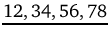
Dim bins are on the left, bright bins on the right. You can have discordance of results, looking in the scopes, either by switching from Histogram to Histogram Bezier or after a conversion between color spaces (with associated change in depth color). The number of bins used depends on the color model bit depth:
All of the bins are scanned when the graph is plotted. What is shown on the graph, in the Compositor window, and finally on the scopes, depends on which plugin is used:
Another difference in behavior is regarding the type of curve, whether Linear or Log:
This diversity also leads to different visual results from Histogram Bezier or Videoscope.
When the color space and the bin size are the same, all of the values increment the indexed bins. But if we start from YUV type edits, the plugin will automatically do the conversion to RGB. When the color is the result of yuv → rgb float conversion, we go from 256 bins of YUV to 65536 bins of RGB Float and the results spread if there are more bins than colors. This is the same effect you see when you turn on smoothing in the vectorscope histogram.
The total pixels for each value is approximately the same, but the max value depends on the color quantization. More colors increment more bins. Fewer colors increment fewer bins. In both cases, the image size has the same number of pixels. So the pixels will distribute into more bins if you go to a higher depth color; those bins will have a lower count. The fewer color case increments the used bins, and skips the unused bins. This sums all of the pixels into fewer bins, and the bins have higher values. That is the rgb vs yuv case, fewer vs more bins are used. To get more consistent visual feedback (and on scopes), the concept of sum was used instead of the maximum number of occurrences (max).
To report something more consistent, the reported value has been changed from the original code to be the sum of the accumulated counts for the bins reporting a pixel bar on the
| 1 | ||||
| 1 | 1 | |||
| 000100 | 3 pixels | vs | 0011000 | 3 pixels |
On the left, the course color model piles all 3 pixels into one bin, max value 3. On the right, the fine color model puts the counts into 2 bins, max 2, sum 3.
So, by reporting the sum the shape of the results are more similar to Bezier.
The CINELERRA-GG Community, 2021